The Data Pane
To open a file containing measured data into ParX choose File > Open Data… (⌥⌘O) to show the Open File dialog.
Select the desired .json, .csv or .tsv file and choose to open the file.
Alternatively, in the Finder, drag and drop a data file directly on the data pane.
Given a model with interface variables you wish to compare with measured data, the measured data points must be linked to the model interface. For each model variable on the left, a data variable must be selected on the right. When there are matching names in de data file header, these will be pre-selected automatically.
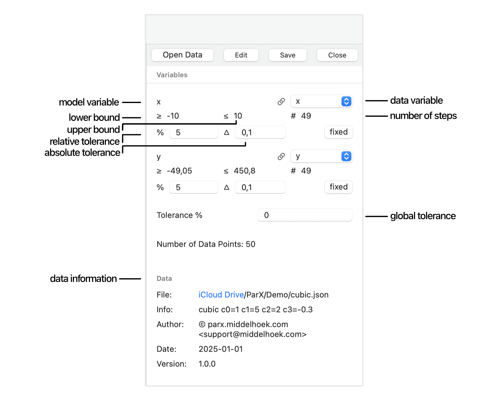
When the data is loaded, its metadata is displayed in the data pane.
The interface variables are shown with the range and number of steps (or number of distinct values minus one) of the linked data variables. In the case of sweep variables, these numbers can be matched in the model pane. The total number of data points is also shown.
When the data is loaded, it is drawn in the same graph as the model. The axes are automatically adjusted to encompass all data points.
The data point markers match the color of the associated model curve and y-axis title.
Error Bars
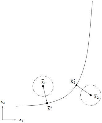
We also need a measure for the accuracy of the match between the model and the data. Therefore, each data point should specify the accuracy of the measurement, or the required accuracy of the model. The clearest representation of this is the error bar.
All data points get error bars; these can be supplied directly in the data file for all coordinates.

Together they define not a data “point” but a data “ellipsoid” centered at the data point.
You will have noticed that in ParX there is no predetermined distinction
between independent and dependent variables.
There can be, but there doesn’t have to be.
An interface variable can be made independent by assigning it a zero error,
either in the data file or through the data pane by selecting its fixed button.
When extracting the model from the data points, the distance between the model curve and a data point is determined with the error ellipsoid as the unit of measure. The distance is one when the model curve touches the ellipsoid.
What is displayed in the Objective field below the graph is the average distance for all data points.
Especially when the model is strongly nonlinear, this principal of determining the shortest distance to the model curve is very beneficial in balancing the influences of data points in the flat and steep regions of the curve, as illustrated here:
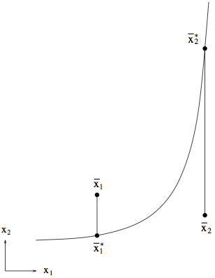
The “weight” of each data point in the result is equalized.
Tolerance Settings
The measurement accuracy is normally provided per data point in the data file.
In case this information is not available, or one wishes to account for additional modeling errors,
the accuracy can be set in the data pane.
A global relative tolerance that applies to all variables can be specified in the Tolerance % field.
Next, each model variable has its own fields for specifying a relative and an absolute tolerance.
When all four tolerances are specified simultaneously, the largest is chosen.
By setting a variable to fixed, the tolerance on that variable for all data points is set to zero. This has the effect of excluding the variable from the distance calculation.
When no error interval is specified, neither in the data file nor in the data pane, or both are set to zero, the calculated distance between the data point and the model curve will be by definition infinite. These data points will be removed from the dataset during optimization, which will reduce the number of “Valid Data Points” below the graph, most probably to zero. This will in turn result in the error message “Insufficient data points” when optimizing.
Therefore, always specify an error interval!
At a minimum through the global Tolerance % field.
Edit the Data
When a data file is already open in the data pane, an editor window will be opened for that data
by pressing the Edit button,
or by the menu command File > Edit Data (⌥⇧⌘O).
The data pane shows the file that will be opened.
When no data file is open in the data pane,
the menu command File > Edit Data… (⌥⇧⌘O)
and the Edit button will show the Open File dialog.
Select the desired .json, .csv, or .tsv file and choose to open the file.
When the data file is openend in the editor window, the data pane will also display its metadata.
Save the Data Settings
The variable selections and tolerance settings can be saved to file for later re-use.
Choose File > Save Data… (⌥⌘S) and supply a file name in the Save File dialog.
The file is saved with the .prxd extension.
The settings can be recreated by choosing File > Open Data… (⌥⌘O) and opening
the file containing them.
Dragging and dropping a .prxd file on the data pane will also reload the data and its settings.
Close the Data
Closing the data will reset the data pane, so a different data file can be openend
without retaining previous settings.
Choose File > Close Data (⌥⌘W), or press the Close button in the
toolbar.
Any open editor windows will lose their connection with the data pane and will no longer auto-reload on save
(unless the same data file is opened again).
Export the Measurement Data
The measurement data can be exported
to a .json file, a .csv file, or a .tsv file.
The .tsv file is UTF16 encoded for better compatibility with older versions Microsoft Excel.
Choose the menu option File > Export Data,
and select the file type, and a file location in the Export File dialog.
This functionality is mainly intended to save the data-part of the result of an optimization. The exported data points will gain two fields, one for the optimization residual (final distance), and one that indicates (with a 1 or a 0) if they belong to the final validity domain (“selected” for CSV, or “grpid” for JSON).
The exported measurement data points will either retain their original error intervals or take their intervals from the specified tolerances in the data pane. In effect, these are the same error intervals that are shown in the graph, and which were used during the optimization.
Create new Measurement Data
For bootstrapping data file creation without the need for an external editor,
there is the option of generating a simple data template,
or making a duplicate of the open data file with a different name or file type.
When no data file is open, the File menu presents the option File > New Data .
This will create an empty data file, using the interface variables of the currently open model for the column names.
When a data file is open, this option is replaced by File > Duplicate Data… .
The newly created data file is automatically opened and can subsequently be modified in the data editor.