The Model Pane
To open a ParX model definition file choose File > Open Model… (⌘O),
or press the Open Model button in the toolbar, to show the Open File dialog.
Select the desired .parx file and choose to open the file.
Alternatively, select the model file in the Finder and choose
Open With in the context menu and select the ParX.app from the App list.
Or, in the Finder, drag and drop a model file directly on the model pane.
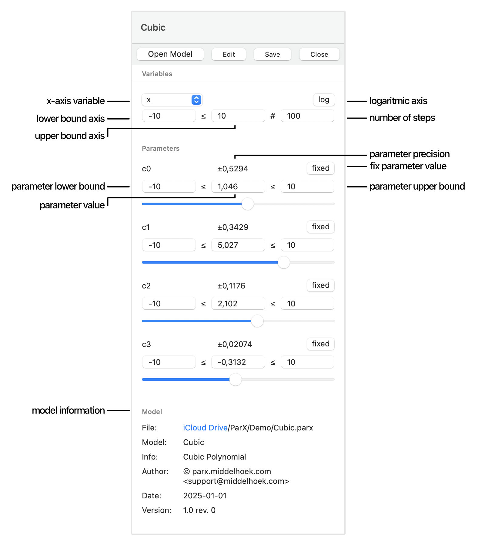
When the model file is opened, the model pane will display the model interface:
the interface variables and the parameters.
The model interface shown here has two variables:
x and y,
and four parameters c0 to c3.
It models a third order polynomial equation.
Before you can plot the model in the graphing pane, the axis’ must be chosen.
The first selected variable is taken as the x-axis of the graph, or sweep variable,
in this example the x variable of the model.
Since the model has only two variables, this places the y variable along the
y-axis.
The plot range for the sweep variable is specified as:
-10 ≤ x ≤ 10 in 100 steps. (Note that this results in 101
points).
The log button determines how the steps are distributed along the x-axis.
In Log mode every decade gets the same number of steps,
which is useful when plotting the model curves on a logarithmic x-axis.
The model parameters each get a value, a lower bound and an upper bound. The slider is connected to the parameter value, and allows it to be varied between the bounds. When the model is first loaded, these fields get set to the default values as specified in the model file.
After extracting the parameter values from the measured data, the parameters acquire an additional field that expresses the precision of the result.
Finally, each parameter has a fixed button that locks its value during optimization.
The graph is drawn as soon as the sweep variables are specified.
The graph is automatically updated when the variable ranges or parameter values are changed. When using the parameter slider to change the parameter value, the model curve(s) and the axes will be animated to show the effect.
When the model file is modified in the background in an external text editor,
the model must be reloaded before the changes are reflected in the model pane and the graph.
Choose File > Reload Model (⌘R).
If the model interface is unchanged (same names), the values will be retained;
else the default values will be restored.
This mechanism allows you to experiment with the model equations interactively.
Edit the Model Definition
The model definition in the .parx file can be inspected and modified
by opening the build-in model editor in a separate window.
Choose File > Edit Model (⇧⌘O),
or press the Edit button in the toolbar.
Save the Model Settings
The interface values of the model can be saved to file for later re-use.
Choose File > Save Model… (⌘S),
or press the Save button in the toolbar, and supply a file name in the Save File dialog.
The file is saved with the .prxs extension.
The settings can be recreated by choosing File > Open Model… (⌘O) and opening
the file containing them.
Opening a .prxs file in the Finder will also load the settings,
as will drag and dropping the file on the model pane.
Close the Model
Closing the model will reset the model pane and unload the model code,
so a different model can be openend without retaining previous settings.
Choose File > Close Model (⌘W),
or press the Close button in the toolbar.
Any open editor windows will lose their connection with the model pane and will no longer auto-reload on save
(unless the same model is opened again).
Export the Model
The interface values can be exported
to a .csv file, a .tsv file, or a .txt file.
The .tsv file is UTF16 encoded for better compatibility with older versions of Microsoft Excel.
Choose File > Export Model,
and select a file type, and location in the Export File dialog.
This functionality is provided mainly for communicating the results of the optimization to other applications, or for archiving said results in a human-readable form.
Export the Simulation Data
The simulated model data (or model curves) can be exported
to a .json file, a .csv file, or a .tsv file.
Choose File > Export Simulation,
and select a file type, and location in the Export File dialog.
This functionality is provided mainly for testing purposes, so when developing a model, its performance can be tested first with synthetic data. Note that the error intervals of the simulated data points will always be zero.
Create a new Model
For bootstrapping model creation without the need for an external editor,
there is the option of generating a simple model template (Cubic Polynomial),
or making a duplicate of the open model under a different name.
When no model is open, the File menu presents the option File > New Model… (⌘N).
When a model is open, this option is replaced by File > Duplicate Model… (⌘N).
Choose a suitable name and location for the model in the Save File dialog.
The newly created model file is automatically opened and can subsequently be modified in the model editor.